Sunday 31 March 2013

Study of Spreading Phenomena in Blog Network Communities

Introduction

Spreading occurs in a network when a an action, information or idea becomes adopted due to the influence of neighbors in the network. The results of studies on diffusion are used in many applications. For example, viral marketing exploits existing social networks and encourages customers to share product information with their friends. The “cascade” diffusion model allows to investigate which individual dynamics lead to global spreading phenomena. A diffusion cascade occurs when information spreads from one node to the rest of the
network through a succession of diffusion events. Cascades have been theoretically analyzed in random graphs using a threshold model.This model uses the community structure of the network.

It has been observed that nodes with common features tend to interact preferentially with each other. These groups of nodes are called communities. Among the various definitions of “community” which exist in the literature, we use the following one: “A community is a set of nodes with common features or interests”. The community structure enables an analysis at different scales: local (individual nodes), global (whole network) and intermediate levels (groups of nodes).

Cascades Computation

1. Data corpus

A blog is composed of a set of posts written at a given time with a body text and references to other pages on the web (for example pictures, videos and websites). The text may contain references to previous posts, from the same blog (auto-citation) or from another blog, by quoting the corresponding URLs, which are called citation links. Citation links are very important as they represent a diffusion of information in the network. Consider a post Pa from blog A and a post Pb from blog B. If Pa contains a reference to Pb, then there is a citation link from Pa to Pb, i.e. Pa cites Pb. In terms of information spreading, we can say that Pa has ’adopted’ Pb’s content or that Pb’s content has been spread towards Pa.
Fig. Blog network community structure

2. Hierarchical Community Structure

The structure may be obtained in two different ways. First, by executing an automatic community detection algorithm. Second, by classifying manually each blog into hierarchical classes. Such a classification is generally hard to obtain due to the large size of datasets, but is very interesting as it is validated manually, unlike automatic classification.The hierarchical community structure considered for this dataset comprises 5 levels: level 0 corresponding to a single community (with all blogs), level 1 with 3 communities called continents (Leisure, Individuality, Society), level 2 with 16 regions, level 3 with 96 territories and finally level 4 with 10,309 individual blogs.In the following, we explain the formalism we will use in the paper. Let a graph G = (V,E), with V a set of nodes and E a set of edges. Our methodology requires a community structure such that each node of V belongs to exactly one community at each level of the tree (more general hierarchical community structures will be considered in the future to allow overlapping communities).

3. Community distance

Given a couple of communities u ∈ Pi and v ∈ Pj , there exists a minimal integer t such that there is a community C in Pt with u ⊂ C and v ⊂ C. We define the community distance of the spreading link (u, v) as:
d(u, v) =[(i − t) + (j − t)]/2


Fig. Community distance example

 
Table: Cascade Shapes ordered by Frequency.
Fig. Largest cascades. All cascades have a number of node >= 40.


References
[1] Abdelhamid Salah Brahim, Bénédicte Le Grand and Matthieu Latapy. Diffusion Cascades: Spreading Phenomena in Blog Network Communities, Parallel Processing Letters 22(1): (2012)
[2] A. S. Brahim, B. L. Grand, L. Tabourier, and M. Latapy. Citations among blogs in a hierarchy of communities: Method and case study. Journal of Computational Science, 2(3):247 – 252, 2011. 
[3] M. Cha, A. Mislove, B. Adams, and K. P. Gummadi. Characterizing social cascades in flickr. In Proceedings of the first workshop on Online social networks, WOSN ’08, pages 13–18, New York, NY, USA, 2008. ACM.
[4] L. P. Cordella, P. Foggia, C. Sansone, and M. Vento. An improved algorithm for matching large graphs. In In: 3rd IAPR-TC15 Workshop on Graph-based Representations in Pattern Recognition, Cuen, pages 149–159, 2001.
[5] M. Girvan and M. E. J. Newman. Community structure in social and biological networks. PNAS, 99(12):7821–7826, 2002.
[6] M. Granovetter. Threshold Models of Collective Behavior. The American Journal of Sociology, 83(6):1420–1443, 1978.


Friday 29 March 2013

Very Complex COMPLEX NETWORKS & Ultimate Complex Network

A Complex Network is a Graph (network) with non-trivial topological features.
Often these features are Not regular and Not random.
So whats difference between a common Graph and Complex Network ?
Only that Complex Network involves Real graphs.

So,I can say

Entire UNIVERSE is a Complex Network containing ~100 Billion Galaxies each containing ~ 100 Billion Stars each containing many planets, meteors, satellites etc around it.
All these are connected to each other by some of the Fundamental Forces discovered and proposed until today. These Individual forces can be Attractive and Repulsive as well depending upon distance between objects.


I Think whether it will be possible that we ll come to know later that there are ~100 Billion Universes like the one we know today, After light travels far beyond and we ll see its actually another BIG BIG BANG going to happen ( as we see all galaxies moving away)?

Also, Human Body is a Complex Network contains BRAIN which is itself a Complex Network.


BRAIN Also Contains ~ 100 Billion Neurons like each Galaxy contain ~100 Billion stars and Universe contains ~100 Billion Galaxies.
There are many type of neurons. They vary in size from 4 microns to 100 microns in diameter and each Neuron communicates with 1,000-10,000 other neurons.
Obviously All Neurons are Connected by some type of edges but, How ?


An ATOM can also be supposed to be a Complex Network too.


There are 36 confirmed fundamental particles, including anti-particles.Twelve of these are the force carrying particles- the photon, the weak force carriers W-, W+, Z0, and the eight gluons. The other 24 are called matter particles and only interact with each other indirectly via the force carriers.These include three types of neutrino, three types of electron-like particles, six types of quark and the 12 associated anti-particles.
So, are some of the subatomic particles themselves Supposed to be Edges Here ?


All Toughest things can be assumed to Belong under Complex Networks.
As they are not  made up of  single basic object. So, its a network involving more than one objects,
and obviously its going to be Complex.

Can we answer 3 questions that I raised in this Blog post ?

With a Large Perspective we see that Almost Everything can be put into the Category you want.

I just imagine a time when we ll be having Projects to Study Entire Universe, Human Body, Human Brain and an Atom under Complex Networks.

They will be VERY COMPLEX COMPLEX NETWORKS because :

There will be types of Nodes. Where one Node can transform to other Node or Group of Nodes   itself(like stars destroy, earth is supposed to be a part of Sun, interactions in an atom).

There will be types of edges like type of forces (where each force can be attractive, repulsive depending upon distances between nodes).

A network where insertion and Deletion of Nodes and Edges takes place itself,even transformation.  We will just need to study and find a useful relation.
But, it really needs lot more advancement in the field of Science and Research.
I just see everything connecting to form an ULTIMATE COMPLEX NETWORK.

References-
1.Wikipedia for Definitions.
2.Google Search for Images.
3.Info you can find anywhere.
4.MY MIND for IDEAS and IMAGINATION.

SORRY for any Mistake or Contradiction(Its just my View and Imagination),
AND, I am not very good at exploiting Blog writing features.
I started thinking the moment i woke up at 5:15 pm and finished writing at 8:25 pm. 

Wednesday 27 March 2013

Deep Learning Artificial Neural Networks and Restricted Boltzmann Machines


What is a Neural Network and Deep Learning in Artificial Neural Networks?
An Artificial Neural Network (ANN) is an information processing paradigm that is inspired by the way biological nervous systems, such as the brain, process information. It is composed of a large number of highly interconnected processing elements (neurones) working in unison to solve specific problems. ANNs, like people, learn by example. An ANN is configured for a specific application, such as pattern recognition or data classification, through a learning process.

Deep learning is part of a broader family of machine learning methods based on learning representations.For example an observation can be better represented in many ways but some representations make it easier to learn tasks of interest.So research in this area works on better representations and how to learn them.

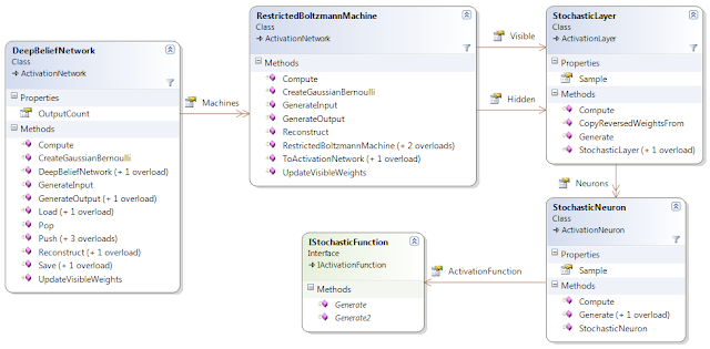
The new version of Accord.NET brings a nice addition for those working with machine learning and pattern recognition : Deep Neural Networks and Restricted Boltzmann Machines

Below is a class diagram for an instance of Deep Neural Network:
Class diagram for Deep Neural Networks in the Accord.Neuro namespace
But why more layers?
The Universal Approximation Theorem (Cybenko 1989; Hornik 1991) states that a standard multi-layer activation neural network with a single hidden layer is already capable of approximating any arbitrary real function with arbitrary precision. Why then create networks with more than one layer?

To reduce complexity. Networks with a single hidden layer may arbitrarily approximate any function, but they may require an exponential number of neurons to do so. Example: Any boolean function can be expressed using only a single layer of AND, OR and NOT gates (or even only NAND gates). However, one would hardly use only this to fully design, let's say, a computer processor. Rather, specific behaviors would be modeled in logic blocks, and those blocks would then be combined to form more complex blocks until we create a all-compassing block implementing the entire CPU.

 By allowing more layers we allow the network to model more complex behavior with less activation neurons; futhermore the first layers of the network may specialize on detecting more specific structures to help in the later classification. Dimensionality reduction and feature extraction could have been performed directly inside the network on its first layers rather than using specific separate algorithms.

Do computers dream of electric sheep?
The key insight in learning deep networks was to apply a pre-training algorithm which could be used to tune individual hidden layers separately. Each layer is learned separately without supervision. This means the layers are able to learn features without knowing their corresponding output label. This is known as a pre-training algorithm because, after all layers have been learned unsupervised, a final supervised algorithm is used to fine-tune the network to perform the specific classification task at hand.


As shown in the class diagram on top of this post, Deep Networks are simply cascades of Restricted Boltzmann Machines (RBMs). Each layer of the final network is created by connecting the hidden layers of each RBM as if they were hidden layers of a single activation neural network.

Now, the most interesting part about this approach will be given now. It is about one specific detail on how the RBMs are learned, which in turn allows a very interesting use of the final networks. As each layer is a RBM learned using an unsupervised algorithm, they can be seen as standard generative models. And if they are generative, they can be used to reconstruct what they have learned. And by sequentially alternating computation and reconstruction steps initialized with a random observation vector, the networks may produce patterns which have been created using solely they inner knowledge about the concepts it has learned. This may be seen fantastically close to the concept of a dream.

Further Reading:

1. Bengio, Y. (2009). Learning Deep Architectures for AI.. Now Publishers.
2. K. Fukushima. Neocognitron: A self-organizing neural network model for a mechanism of pattern recognition unaffected by shift in position. Biological Cybernetics, 36(4): 93-202, 1980.
3. M Riesenhuber, T Poggio. Hierarchical models of object recognition in cortex. Nature neuroscience, 1999.
4. S. Hochreiter. Untersuchungen zu dynamischen neuronalen Netzen. Diploma thesis, Institut f. Informatik, Technische Univ. Munich, 1991. Advisor: J. Schmidhuber
5. S. Hochreiter, Y. Bengio, P. Frasconi, and J. Schmidhuber. Gradient flow in recurrent nets: the difficulty of learning long-term dependencies. In S. C. Kremer and J. F. Kolen, editors, A Field Guide to Dynamical Recurrent Neural Networks. IEEE Press, 2001.
6. Hochreiter, Sepp; and Schmidhuber, Jürgen; Long Short-Term Memory, Neural Computation, 9(8):1735–1780, 1997
7. http://blogs.technet.com/b/next/archive/2012/06/20/a-breakthrough-in-speech-recognition-with-deep-neural-network-approach.aspx#.UVJuIBxHJLk


Sunday 24 March 2013

Analysing Social Networks to predict the future !

Online Social networks enable us to express ourselves and reach out in an inexpensive and extremely convenient manner. Twitter recently announced a staggering 200 million active users! Facebook claims to have 1 billion. Such widespread use of online social networks provides researchers with a firehose of well organized data. Now, what does a researcher do with data? No points for guessing. He/she analyses it!

Some research which I will talk about, analyse it to make predictions about various things - Movie Box-Office, Stock Prices, Trending Topics, Election Results, etc.

However before we discuss about it, I would like to point out to you that all of this research assumes that buzz on the Web reflects popularity and buzz in the real world. To what extent this premise is valid, is another interesting research topic, but let's not go into it right now.

Lets back to the topic of predicting the future. [1] describes a procedure to identify trends through semantic social network analysis. 

A "Web Buzz Index" is calculated for "concepts" which are input in the form of phrases. "Concepts" may be names of politicians, brands, or general topics of interest. To do this, they extend the concept of betweenness centrality of actors in social networks to semantic networks of concepts.  Trends are measured by tracking a concept’s relative importance in a relevant information sphere - Web, blog, or online forums. Betweenness centrality of the concept is used as a representative of the relative importance of a concept in the information sphere.

To build the semantic social network in an information sphere, "degree of separation search" is used. Degree of separation search works by building a two mode network map displaying the linking structure of a list of Web sites or blog posts returned in response to a search query, or the links among posters responding to an original post in an online forum.

Degree of separation search can be employed to compare the relative importance of various concepts. The figure below shows the comparison of relative importance of the concepts “gun control”, “abortion”, “gay marriage”, and “Iraq war”. So, The idea is that the importance of an individual concept depends on the linking structure of the temporal network and the betweenness of the other concepts in the network.


Further analysis which [1] presents is the social network of blog posts right after the US presidential elections Nov 4, 2008. The blogs talking about McCain form a far more compact cluster, at the very bottom with a tightly interlinked structure. The democratic blogs, linking to Obama, are much wider spread out, and also exhibit fewer interconnecting links, reflecting the wider political interests of the voters supporting Obama.


In [1], the researchers have applied their complete procedure collected data over 213 days (April, 1st 2008 until October, 30th 2008) on 21 stock titles on Yahoo! Finance. The results (for stock prices of Goldman Sachs) as we can see below, show a promising correlation between the web buzz and real world stock prices.


Thus, it is evident from the results of the existing research, that social networks can be used as an indicator of the future. The analysis of sentiments can reveal the results of people driven events like the success of a movie, elections, market fluctuations, and what not!

Further Reading:

1.     Gloor, Peter A., et al. "Web Science 2.0: Identifying Trends through Semantic Social Network AnalysisComputational Science and Engineering, 2009. CSE'09. International Conference on. Vol.4. IEEE, 2009
2.     Asur, Sitaram, and Bernardo A. Huberman. "Predicting the Future With Social Media" arXiv preprint arXiv:1003.5699 (2010)
3.     Yu, Sheng, and Subhash Kak. "A Survey of Prediction Using Social Media" arXiv preprint arXiv:1203.1647 (2012)
4.     Wasserman, Stanley, and Katherine Faust. Social network analysis: Methods and applications. Vol. 8. Cambridge university press, 1994.
5.     Data And Text Mining Of Financial Markets Using News and Social Media (Dissertation by Zhichao Han)

Thursday 21 March 2013

Transforming Time Series into Complex Networks

In this post we will look into the transformations from time series data to the domain of complex networks which will allow us to characterise the dynamics underlying the time series in terms of topological features of the complex network. We will see that the constructed graph inherits several properties of the series in its structure. Thereby, periodic series convert into regular graphs, and random series do so into random graphs. Moreover, fractal series convert into scale-free networks, enhancing the fact that power law degree distributions are related to fractality, something discussed by Ayush Goel in his post ‘Fractality in Complex Networks’ recently.

We will look into a simple and fast computational method, the visibility algorithm, to convert a time series into a graph. The main idea is to study to which extent the techniques and focus of graph theory are useful as a way to characterize time series. The key question is to know whether the associated graph inherits some structure of the time series, and consequently whether the process that generated the time series may be characterized by using graph theory.

Visibility Algorithm for Time Series :
First, we consider periodic series. For illustrative purposes, in Fig. 1 we present a scheme of the visibility algorithm. In the upper zone we plot the first 20 values of a periodic series by using vertical bars (the data values are displayed above the plot). Considering this as a landscape, we link every bar (every point of the time series) with all those that can be seen from the top of the considered one (gray lines), obtaining the associated graph (shown in the lower part of the figure). In this graph, every node corresponds, in the same order, to series data, and two nodes are connected if visibility exists between the corresponding data, that is to say, if there is a straight line that connects the series data, provided that this “visibility line” does not intersect any intermediate data height.


Fig. 1.

                                                                       Fig. 1


More formally, we can establish the following visibility criteria: two arbitrary data values(ta, ya) and (tb,  tb) will have visibility, and consequently will become two connected nodes of the associated graph, if any other data (tc, yc) placed between them fulfills: 

 Formula
                                                

We can easily check that by means of the present algorithm, the associated graph extracted from a time series is always
1.      Connected: each node sees at least its nearest neighbors (left and right).
2.      Undirected: the way the algorithm is built up, there is no direction defined in the links.
3.      Invariant under affine transformations of the series data: the visibility criterion is invariant under rescaling of both horizontal and vertical axes, and under horizontal and vertical translations  (see Fig. 2).


Fig. 2.

Fig. 2

The visibility graph of a time series remains invariant under several transformation of the time series. (a) Original time series with visibility links. (b) Translation of the data. (c) Vertical rescaling. (d) Horizontal rescaling . (e) Addition of a linear trend to the data. As can be seen in the bottom diagram, in all these cases the visibility graph remains invariant.

The example plotted in Fig. 1 is a periodic series with period 4. The associated visibility graph is regular, as long as it is constructed by periodic repetition of a pattern. The degree distribution of this graph is formed by a finite number of peaks related to the series period, much in the vein of the Fourier power spectrum of a time series. Generically speaking, all periodic time series are mapped into regular graphs, the discrete degree distribution being the fingerprint of the time series periods. In the case of periodic time series, its regularity seems therefore to be conserved or inherited structurally in the graph by means of the visibility map.

Random Graphs :
As an opposite to periodic series, in a second step we will tackle a series R(t) of 10^6 data values extracted from an uniform distribution in [0, 1]. Although one would expect in a first moment a Poisson degree distribution in this case [as for uncorrelated random graphs (1)], a random time series has indeed some correlation, because it is an ordered set. In fact, let k(t) be the connectivity of the node associated with the data t. If  k(t) is large (related to the fact that the data have a large value and that consequently they have large visibility), one would expect that k(t+1) would be relatively small, because the time series is random and two consecutive data values with a large value are not likely to occur. It is indeed because of these “unlikely” large values (the hubs) that the tail of the degree distribution deviates from the Poisson distribution.
Two large values in the series data can be understood as two rare events in the random process. The time distribution of these events is indeed exponential (2), therefore we should expect the tail of the degree distribution in this case to be exponential instead of Poissonian , as long as the form of this tail is related to the hub's distribution.


Fig. 3.

                                                                             Fig. 3 

In the left side of Fig. 3 we depict the first 250 values of R(t) . In the right side we plot the degree distribution P(k) of its visibility graph (plotted in semilog). The tail of this distribution fits an exponential distribution quite well, as expected.

Therefore, order and disorder structure in the time series seem to be inherited in the topology of the Visibility Graph Network. These algorithms provide a new way of studying time series in the complex networks domain and equip us with a wide range of statistical measures.


REFERENCES
(1) Bollobás B (1998) Modern Graph Theory (Springer, New York).
(2) Feller W (1971) An Introduction to Probability Theory and Its Applications (Wiley, New York).
(3) arxiv.org/abs/1208.6365
(4) http//www.eie.polyu.edu.hk/~ensmall/pdf/COMPLEX09-1.pdf

Wednesday 20 March 2013

How easy is it to 'control' a complex network?

Before I discuss the above question, let me first ask, how desirable is it to control complex networks around us? This one is easily answerable. Think of the complex networks within our own bodies - the biological systems. It is not surprising to know that targeting certain 'spots' in the complex biological systems within us can give us a great control on governing metabolism, however sophisticated. Figuring out how bacterial metabolic networks are controlled could help biologists identify new and easy targets for antibiotics by determining which points in the network are the most vulnerable.
Ability to control networks also means that trouble could be caused more easily. Consider a situation where someone fond of mischief knows exactly what minimal set of power lines to trip to put off electricity for the whole city.
The proof of our understanding of complex systems is very much reflected in our ability to control them. In this post, I will talk about some basic jargon of network controllability and vulnerability.

Control Theory

According to control theory, a system is controllable, if it can be driven from any intial state to any desired final state by varying certain inputs.
Assuming linear control systems, described by the following state equation,

                                                           x˙(t) = A.x(t)+B.u(t)


which is the state of a system with N nodes.  Here, x is the state vector and u is the input (control) vector. A is the NxN adjacency matrix of the network representing the system. B is the NxM input matrix which identifies the nodes where the input signals are imposed. The state of each node at each time step is controlled by a linear combination of the elements of the input vector. The system defined by the above equation is controllable if and only if the controllability matrix,

                                                               C = [B AB A2B] 

which is a NxNM matrixhas full rank, i.e. Rank(C) = N.
This controllability rank condition is given by Kalman.
The critical question here is how do we find out the minimum number M (M < N) of different signals that offer full control over the network? Kalman's theory is only feasible for small networks, while for large real networks, it is very hard to compute the rank of C, since C is an incredibly large matrix.
This is where Liu, Slotine and Barabasi come to rescue.

Liu, Slotine and Barabasi

Slotine, an MIT researcher has come up with a new computational model that can analyze a wide variety of complex networks, ranging from biological to social networks. His work was motivated to reveal the critical points that could be used in controlling the entire system, and ideally, this fraction of driver nodes is supposed to be low, for better ease and control.

Slotine and his co-authors devised a computer algorithm that can generate a controllability structure for any complex network. The red points are 'driver nodes,' which can control the rest of the nodes (green).

They showed that minimum number of nodes (driver nodes) can be found out in the 'maximum' matching of the network. In graph theory, the maximum matching of a directed network is the maximum set of links that do not share start and end nodes, and a node is matched if it is the end of a directed link in the maximum matching set, otherwise it is unmatched.
For sparse networks, such as gene regulatory networks, they found the number to be high, around 80%, implying the difficulty of control. For dense networks, such as neuronal networks, the number was about 10%.
Well, what determines the number of driver nodes? An intuitive guess would be our favorite property, the degree distribution, which describes the number of connections per node. This is indeed the case - the knowledge of degree distribution can very much help in estimating the number.


           An example of maximum matching and network control, via driver nodes

Vulnerability

It is generally assumed that when a node is attacked, its edges are removed from the network, but the node itself is still in the network, so the size of the network is unchanged after attacks.
Intuitively, network controllability is supposed to decrease after attacks, which is reflected as increase in the number of driver nodes.

A single node attack may be a random one, or a degree-based attack. Degree-based attacks are
more efficient in attacking the network controllability rather than random attacks, reason being that degree based attacks have more edges removed from the network at each time step, which indicates that most likely more matched links are removed in the degree-based attacks at each time step, compared to that of the random attacks. As a result, the network controllability decreases faster which reflects in the need for more control signals or driver nodes to control the network. Interested readers should follow up the references.

A very good analogy could be that of power grids. The node with largest load will obviously cause greatest disruption on failure.

In conclusion,  the area of control of networks is very important one, and although much work has been done in this area, there are a number of open problems of outstanding practical signifinance that budding network researchers can take up. For example, in context of vulnerability, defense strategies are very important and need further research.


References:

(1) MIT News: How to control complex networks - http://web.mit.edu/newsoffice/2011/network-control-0512.html

(2) Controllability of Complex Networks - Yang-Yu Liu, Jean-Jacques Slotine & Barabasi

(3) Robustness Analysis of Network Controllability - Cun-Lai Pua, Wen-Jiang Peib, Andrew Michaelsond

Monday 18 March 2013

Dr Jekyll and Mr Hyde : Detecting Sybils in Social Networks

Prologue

In December 2002, ZDNet, a famous technology website conducted a poll in the United Kingdom to find out what platform their readers preferred to build web services. By the end of December, a large majority of those (nearly half the total sample) had responded saying they were planning to use Java. Only 21.5 percent said they planned to use Microsoft .Net - less than the figure (23.5 percent) planning to use neither. But by the time the poll closed, on 5 January, the position had dramatically changed, with three quarters of voters claiming to be implementing .Net. ZDNet UK logs revealed rather obvious vote rigging, including a large number of people who made attempts at multiple voting using fake logins despite that being blocked by the poll scripts ( The one that takes the cake made a whopping 228 attempts to vote)[1].Sounds like a scene straight from a conspiracy movie, doesn't it? Sadly, this is case of fact imitating fiction.

The problem of fake identities, or Sybils as they are known as*, is not a new one,neither in the real nor the virtual world, but with the rise of online social networks, the need to detect such Sybils and separate the fake from the real has only risen since fakes can introduce spam, manipulate online rating, or exploit knowledge that they have extracted from the network. There have been several approaches to detect Sybils and today I'll discuss one of these approaches, known as SybilRank[2] that detects suspicious accounts in a social network based on a social-graph with bidirectional relationship.


The Concept

A visual overview of Sybil nodes and attack edges

SybilRank works on an undirected social graph with the assumption that non-Sybil nodes are well-connected. It also assumes that Sybils establish attack edges to non-Sybil nodes, which are limited in number, due to the difficulty of soliciting and maintaining reciprocal social relationships and Sybils randomly attach attack edges to non-Sybils.
SybilRank uses a power iteration method similar to the one used in PageRank and ranks users according to suspiciousness. This works as follows :

1) The iterations start with a set of trust-seeds (profiles/user which we know for sure are non-Sybils) with all of them assigned an initial and equal amount of “trust”, which is a numerical value whose sum across all nodes remains constant throughout the iterations.

2) In each iteration, every node performs a calculation similar to the one used in calculating PageRank. It considers the trust of all its neighbours and updates its trust by summing all these trust values. Thus if the trust value of a node v after (i-1) iterations is Ti-1v, then 


The above iterations are not allowed to go to completion. Instead they are terminated early (say after log(n) iterations), after which you get a ranking based on the trust values of the nodes. This ranking is prepared by degree-normalizing the trust value since it removes the bias towards degrees (which contributes to this algorithms better perfomance). Now why does this work? Re-read the assumption that states that attack-edges are limited in number. Hence, trust can flow to the Sybil nodes through a very limited number of edges, thus condemning them to the nadir of the rankings list.

The Case of Communities

We know that almost all social networks have communities embedded within them and these communities usually have a very limited number of edges connecting them. If the above algorithm, chooses the trust seeds from a selected number of communities, then there is a very high chance of marking nodes from other communities as Sybil-nodes incorrectly. To overcome this, the trust seeds are distributed across possible communities to ensure fairness. The method used by the creators of SybilRank is to start by discovering communities using the Louvain method[3] and then seed nodes in each discovered community.


My $0.02

The SybilRank algorithm is an innovative and efficient algorithm, and has taken a lot of forward steps as compared to previous algorithms by its features such as its use of power-iteration-computed landing probability as opposed to random walk traces (SybilLimit[4]). As compared to other power-iteration algorithms (EigenTrust[5]), its better performance was put down to the two features, one the early-termination and the second was the degree-normalization. However, the last call after applying any such algortithms still cannot be automated since these algorithms only produce a list that has to be manually verified which is still a tedious process that consumes a lot of manpower. Also this algorithm cannot successfully detect Sybils which attack the non-Sybils in a planned manner, or by targeting a large number of non-Sybils. If possible, I'll discuss these and various other methods for Sybil detection or prevention of Sybil attacks in a future blog-post.

References:

[1] .Net vote rigging illustrates importance of Web services - http://www.zdnet.com/net-vote-rigging-illustrates-importance-of-web-services-3002102244/
[2] Aiding the Detection of Fake Accounts in Large Scale Social Online Services, Qiang Cao, Michael Sirivianos, Duke University, Xiaowei Yang, Tiago Pregueiro.
[3] Fast Un-folding of Communities in Large Networks,V. D. Blondel, J.-L. Guillaume, R. Lambiotte, and E. Lefebvre
[4] SybilLimit : A Near Optimal Social Network Defense Structure Against Sybil Attacks, Haifeng Yu,  Philip Gibbons, Michael Kaminsky, Feng Xiao
[5] The EigenTrust Algorithm for Reputation Management in P2P Networks : Sepandar D. Kamvar, Mario T. Schlosser, Hector Garcia-Molina


Notes:

* - Interestingly, the name Sybil comes from a book of the same name, wherein the titular character suffered from dissociative identity disorder, and manifested no less than 16 different personalities.


Saturday 16 March 2013

Query Dependent Ranking

WHY?

 - The first question that might come to your mind is what is the need of this 'Query Dependent    Ranking', when we are living in the age of Google which uses Page Rank which is Query Independent Ranking. 


Brief Overview of Query Independent Ranking

- The goal of query-independent ranking is to assign a score to each page that measures the intrinsic quality or authority of the page. According to the assumptions behind hyperlink analysis a page A to which many hyperlinks point is likely to be more authoritative than a page to which few hyperlinks
point. However, an approach that just counts the hyperlinks can be easily manipulated and it ignores the fact that the pages pointing to A also can be different quality. Brin and Page proposed instead the following recursive approach: The authority score, called PageRank, of a page A depends
on the authority scores of the pages pointing to B. More specifically, the PageRank R(A) of page A is defined as
R(A) = δ/n + (1 − δ) X hyperlink (B,A) R(B)/outdegree(B),
where δ is a constant usually chosen between 0.1 and 0.2, n is the number of pages in the collection, and outdegree(B) is the number of hyperlinks on page B.

Problem with Query Independent Ranking

Considering the large differences between different queries, it might not be the best choice to use a
single ranking function to deal with all kinds of queries. Instead, one may achieve performance gain by leveraging the query differences. To consider the query difference in training, one can use a query-dependent loss function. To further consider the query difference in the test process, a query-dependent ranking function is needed. Several ways of learning a query-dependent ranking function are reviewed in this chapter, including query classification-based approach, query clustering-based approach, nearest neighbor-based approach, and two-layer learning-based approach.

- Queries in web search may vary largely in semantics and the users’ intentions they represent, in forms they appear, and in number of relevant documents they have in the document repository. For example, queries can be navigational, informational, or transactional. Queries can be personal names, product names, or terminology. Queries can be phrases, combinations of phrases, or natural language sentences. Queries can be short or long. Queries can be popular (which have many relevant
documents) or rare (which only have a few relevant documents). If one can successfully leverage query differences in the process of learning to rank, one may have the opportunities to achieve better ranking performances in both training and test processes.

QUERY DEPENDENT SEARCH comes to the rescue!!!

In query-dependent ranking each page is assigned a score that measures its quality as well as its relevance to the user query. The basic idea is to build for each query a small subgraph of the whole web graph, called a neighborhood graph, and perform hyperlinks analysis on it. Carriere and Kazman propose the following approach to construct a neighborhood graph: 
  1. A start set of documents matching the query is determined.Specifically, they propose to choose the top 200 matches returned by a search engine for the query. 
  2. This start set is augmented by its “neighborhood”, which is the set of documents that either contain hyperlinks to a document in the start set or are referenced by documents in the start set. 
  3. Each document in the start set and its neighborhood is modeled by a node in the neighborhood graph. Two nodes are considered to be unaffiliated if they are on different web hosts. There exists an edge from node A and node B if and only if A and B are unaffiliated and document A has a hyperlink to document B. Edges between affiliated nodes are not allowed to limit the manipulation of the score. Given the neighborhood graph various ranking approaches were suggested. Carriere and Kazman proposed simply to count the number of hyperlinks in the neighborhood graph.

Problem with Carriere and Kazman approach

- Computing the PageRank on the neighborhood graph produces a very similar ranking, mostly because the neighborhood graph is usually small (on the order of a thousand nodes) and the impact of the global web is lost. 

Now Kleinberg!!

-Kleinberg proposed another approach of ranking pages in the neighborhood graph. It assumes that a topic can be roughly divided into pages with good content, called authorities, and pages with good references, called hubs. To determine the authorities and hubs the algorithm iteratively computes hub and authority scores for each node. The intuition is that high authority nodes should be pointed to by many hubs and especially by the good hubs. Good hub nodes on the other side should point to high authority nodes.
This leads to the following algorithm on a neighborhood graph with node set V and edge set E. 
  1. For every node A in V , initialize its hub score Hub[A] to 1 and its authority score Aut[A] to an arbitrary value.
  2. While the vectors Hub and Aut have not converged:
  • For all A in V , Aut[A] = P(B,A)∈E Hub[B]
  • For all A in V , Hub[A] = P(A,B)∈E Aut[B]
     3.  Normalize the Hub and Aut vectors to 1.

- Using linear algebra it is straightforward to show that the Hub and Aut vectors will eventually converge, but no bound on the number of iterations required for convergence is known. In practice, they converge quickly. 
- The success of this approach is very dependent on the quality of the neighborhood graph. Specifically, the neighborhood graph needs to contain high-quality pages on the query topic. 
- If the majority of the pages is on a different topic then topic drift can occur where the top authority pages belong to the different topic. 
- Another disadvantage is that adding a few edges to the neighborhood graph can considerably change the top authority and hub pages since the neighborhood graph is usually fairly small. Thus, there is the risk of manipulation of the results by adding just a few edges. 

Many improvements and generalizations have been suggested to the above two algorithms. (for eg [2] and [3] in references. 


References:

  1. B. Amento, L. Terveen, and W. Hill. Does authority mean quality? predicting expert quality ratings of web documents. In Proceedings of the 23rd International ACM SIGIR Conference in Research and Development in Information Retrieval (SIGIR 00), pages 296–303, New York, USA, 2000. ACM Press.
  2. K. Bharat and M. Henzinger. Improved algorithms for topic distillation in hyperlinked environments. In Proceedings of the 21st International ACM SIGIR Conference on Research and Development in Information Retrieval (SIGIR’98), pages 111–104, 1998.
  3. P. Boldi, M. Santini, and S. Vigna. Pagerank as a function of the damping factor. In Proceedings of the 14th International World Wide Web Conference (WWW2005), pages 557–566, May 2005.
  4. Bian, J., Liu, T.Y., Qin, T., Zha, H.: Ranking with query-dependent loss for web search. In:Proceedings of the 3rd International Conference on Web Search and Web Data Mining (WSDM 2010), pp. 141–150 (2010)
  5. Hyperlink Analysis on the World Wide Web Monika Henzinger Google Inc 8002 Zurich, Switzerland monika@google.com.
  6. Broder, A.: A taxonomy of web search. SIGIR Forum 36(2), 3–10 (2002)


Friday 15 March 2013

Complexity of Nature

Complexity of Nature


Ideas thus made up of several simple ones put together, I call complex; such as beauty, 
gratitude, a man, an army, the universe - John Locke, English Philosopher (1632-1704)

Introduction

Throughout human history the complex patterns that appear everywhere in nature have been cause for wonder and fascination. We are puzzled, for example, about how intricate snowflakes can form in plain air, and our minds boggle at the complexity of even the simplest living systems. Scientists have learned a great deal about natural pattern formation in recent years. Mostly, however, we have discovered how very much remains to be understood.


Think about ice ferns on a window a frosty winter day. We know that the molecules that water is made from are quite simple. They behave like small bricks that attract each-other.Nevertheless, they form ice ferns, like those on the picture, when they are deposited on a cold substrate. The ice ferns are a direct result of the molecules' tendency to be deposited next to each other, that is to say their relative attraction. What appears to be simple step by step is still the origin of complicated shapes. 
The ice ferns on the picture are from a car window and look 
almost like living plants.The point is that we could not have guessed these forms only by looking at a single molecule. A vast number of molecules are needed to form an ice fern, typically on the order of billions. This is an example showing that a simple rule, repeated many times over, gives a complicated but identifiable result, where the whole is more than the sum of its constituents.

The ice ferns build themselves up step by step as the water molecules deposit on the cold glass surface. This is complexity. There is no architect behind the ice ferns. The secret behind the ice ferns' complicated form must be hidden in the interplay between the individual water molecules. 

The question is how. Nature is loaded with similar examples that simple rules on a small scale give complex results on a level visible to the human eye. These include cumulus clouds on a summer day, an oak tree's thousand branches, waves on an agitated sea, or the stripes of the tiger.


Where to Start the Description? 


Our understanding of a complex system depends on at which level we start to describe it. We may look at our ice ferns in an electron microscope, which shows single molecules, and on this scale they appear regular and simple. Looked at by eye from a close range, complexity emerges, but at a longer distance, say 20 meters, only a white spot is seen, which again is rather simple.Complex systems may also be considered as units, which can be pieced together to larger systems. Many trees make a forest; many clouds make a cloud cover, and so on. In the case of the forest, a tree plays the role of a component -- a green dot or a green particle in a forest that is complicated at some level. Maybe it grows along the coastline shaped by straights and bays, or maybe there is room for rivers winding through the landscape. From a far distance the forest itself can play the role as "particle", which together with all the other forests on the earth constitutes a substantial part of the earth's biosphere. 

Description of Complex Systems


A main challenge in the study of complex systems is to find a description by numbers 

(preferably not too many numbers). Only when measurements can be compared with 
theoretical calculations, and vice versa, are we able to judge whether an idea is right or wrong. 

In order to do that, we need numbers. A famous class of observations, which let themselves describe by a single number, are fractals. When something is fractal it consists of parts of many different lengths, and we can put a number on how many of the smaller pieces there are in comparison to how many there 

are of the larger pieces. This number is called the fractal dimension. For instance, in a cup of coffee, see 
Figure , there exist large, medium and small bubbles. If the relative amounts of these bubbles may be described by a number, then the bubbles may have a fractal dimension.


However, not all complex structures have a fractal dimension.

Do you see what the image to the right in Figure shows? It 
shows a 
cut through red cabbage. The pattern is complex yet identifiable to the observer, but it is not clear that one 
may put a number on it.


Wiring diagrams for complex networks

a, Food web of Little Rock Lake, Wisconsin, currently the largest food web in the primary literature5. Nodes are functionally distinct 'trophic species' containing all taxa that share the same set of predators and prey. Height indicates trophic level with mostly phytoplankton at the bottom and fishes at the top. Cannibalism is shown with self-loops, and omnivory (feeding on more than one trophic level) is shown by different coloured links to consumers. (Figure provided by N. D. Martinez). b, New York State electric power grid. Generators and substations are shown as small blue bars. The lines connecting them are transmission lines and transformers. Line thickness and colour indicate the voltage level: red, 765 kV and 500 kV; brown, 345 kV; green, 230 kV; grey, 138 kV and below. Pink dashed lines are transformers. (Figure provided by J. Thorp and H. Wang). c, A portion of the molecular interaction map for the regulatory network that controls the mammalian cell cycle6. Colours indicate different types of interactions: black, binding interactions and stoichiometric conversions; red, covalent modifications and gene expression; green, enzyme actions; blue, stimulations and inhibitions. (Reproduced from Fig. 6a in ref. 6, with permission. Figure provided by K. Kohn.)

Wings, Horns, and Butterfly Eyespots: How Do Complex Traits Evolve?

Throughout their evolutionary history, organisms have evolved numerous complex morphological, physiological, and behavioral adaptations to increase their chances of survival and reproduction. Insects have evolved wings and flight, which allowed them to better disperse [2], beetles have grown horns to fight over females [3], and moths and butterflies have decorated their wings with bright circles of colored scales to scare off predators [4]. The way that most of these and other adaptations first evolved, however, is still largely unknown. In the last two decades we have learned that novel traits appear to be built using old genes wired in novel ways [5], but it is still a mystery whether these novel traits evolve when genes are rewired de novo, one at a time, into new developmental networks, or whether clusters of pre-wired genes are co-opted into the development of the new trait. The speed of evolution of novel complex traits is likely to depend greatly on which of these two mechanisms underlies their origin. It is important, thus, to understand how novel complex traits evolve.
Complex traits require co-ordinated expression of many transcription factors and signaling pathways to guide their development. Creating a developmental program de novo would involve linking many genes one-by-one, requiring each mutation to drift into fixation, or to confer some selective advantage at every intermediate step in order to spread in the population. While this lengthy process is not completely unlikely, it could be circumvented with fewer steps by recruiting a top regulator of an already existing gene network, i.e., by means of gene network co-option. Subsequent modifications of the co-opted network could further optimize its role in the new developmental context.


References


Ball, Philip: Made to Measure: New Materials for the 21st Century, Princeton, New Jersey: Princeton University 
Press 1997 
 Ball, Philip: The Self-made Tapestry: Pattern formation in nature, NewYork: Oxford University Press 1999
 Ball, Philip: Critical mass; How one thing leads to another, Arrow books 2005
 Ball, Philip: Flow; Nature's Patterns: A Tapestry in Three Parts, Oxford university press 2009 
 Barabasi, A-L.: Linked; How everything is connected to everything else and what it means for business, science 
and everyday life, Plume 2003 
 Bentley, P.J.: Digital Btioiogy. The creation of life inside computers and how it will affect us, London Headline 
Books Publishing 2001 
 Benyus, J.M.: Biomimicry: Innovation inspired by nature, NewYork: W. Morrow and ComPany Inc. 1997